Jupyterとpandasdmxを使用して、OECDの全国内交通機関インフラ投資に対する国内水路インフラ投資割合データを取得する

Jupyterとpandasdmxを使用して、OECDの全国内交通機関インフラ投資に対する国内水路インフラ投資割合(=Share of inland waterways infrastructure investment in total inland transport infrastructure investment)データを取得しグラフ表示するには、以下のコードを実行します。

〇出力グラフ

〇コード

from pandasdmx import Request
import matplotlib.pyplot as plt

oecd = Request('OECD')
countries="FRA+ITA+HRV"
data_response = oecd.data(resource_id='ITF_INDICATORS', key=countries + ".IND-INFR-IWINV-SHARE/all?startTime=2000&endTime=2016")
oecd_data = data_response.data

df = data_response.write(oecd_data.series, parse_time=True)
df = df.unstack(level=0).to_frame()
df.columns=['Share of inland waterways infrastructure investment']
df = df.reset_index()
df = df[["COUNTRY", "TIME_PERIOD", "Share of inland waterways infrastructure investment"]]
df.set_index(["COUNTRY", "TIME_PERIOD"], inplace=True)
ax = df.unstack(level=0).plot()
plt.xticks(rotation=90)
plt.legend(loc='best')
plt.show()

〇元データ
Indicators
https://stats.oecd.org/Index.aspx?DataSetCode=ITF_INDICATORS


○関連情報
・Pandasdmxに関する他の記事はこちらを参照してください。

Jupyterとpandasdmxを使用して、OECDの全国内交通機関インフラ投資に対する道路インフラ投資割合データを取得する

Jupyterとpandasdmxを使用して、OECDの全国内交通機関インフラ投資に対する道路インフラ投資割合(=Share of road infrastructure investment in total inland transport infrastructure investment)データを取得しグラフ表示するには、以下のコードを実行します。

〇出力グラフ

〇コード

from pandasdmx import Request
import matplotlib.pyplot as plt

oecd = Request('OECD')
countries="FRA+ITA+AUS"
data_response = oecd.data(resource_id='ITF_INDICATORS', key=countries + ".IND-INFR-RDINV-SHARE/all?startTime=2000&endTime=2016")
oecd_data = data_response.data

df = data_response.write(oecd_data.series, parse_time=True)
df = df.unstack(level=0).to_frame()
df.columns=['Share of road infrastructure investment']
df = df.reset_index()
df = df[["COUNTRY", "TIME_PERIOD", "Share of road infrastructure investment"]]
df.set_index(["COUNTRY", "TIME_PERIOD"], inplace=True)
ax = df.unstack(level=0).plot()
plt.xticks(rotation=90)
plt.legend(loc='best')
plt.show()

〇元データ
Indicators
https://stats.oecd.org/Index.aspx?DataSetCode=ITF_INDICATORS


○関連情報
・Pandasdmxに関する他の記事はこちらを参照してください。

Jupyterとpandasdmxを使用して、OECDの全国内交通機関インフラ投資に対する鉄道インフラ投資割合データを取得する

Jupyterとpandasdmxを使用して、OECDの全国内交通機関インフラ投資に対する鉄道インフラ投資割合(=Share of rail infrastructure investment in total inland transport infrastructure investment)データを取得しグラフ表示するには、以下のコードを実行します。

〇出力グラフ

〇コード

from pandasdmx import Request
import matplotlib.pyplot as plt

oecd = Request('OECD')
countries="FRA+ITA+AUT"
data_response = oecd.data(resource_id='ITF_INDICATORS', key=countries + ".IND-INFR-RLINV-SHARE/all?startTime=2000&endTime=2016")
oecd_data = data_response.data

df = data_response.write(oecd_data.series, parse_time=True)
df = df.unstack(level=0).to_frame()
df.columns=['Inland waterways infrastructure investment']
df = df.reset_index()
df = df[["COUNTRY", "TIME_PERIOD", "Inland waterways infrastructure investment"]]
df.set_index(["COUNTRY", "TIME_PERIOD"], inplace=True)
ax = df.unstack(level=0).plot()
plt.xticks(rotation=90)
plt.legend(loc='best')
plt.show()

〇元データ
Indicators
https://stats.oecd.org/Index.aspx?DataSetCode=ITF_INDICATORS


○関連情報
・Pandasdmxに関する他の記事はこちらを参照してください。

Jupyterとpandasdmxを使用して、OECDの国内水路インフラ投資(住民一人あたりのUSD額)データを取得する

Jupyterとpandasdmxを使用して、OECDの国内水路インフラ投資(住民一人あたりのUSD額)(=Inland waterways infrastructure investment in current USD per inhabitant)データを取得しグラフ表示するには、以下のコードを実行します。

〇出力グラフ

〇コード

from pandasdmx import Request
import matplotlib.pyplot as plt

oecd = Request('OECD')
countries="FRA+ITA+BEL"
data_response = oecd.data(resource_id='ITF_INDICATORS', key=countries + ".IND-INFR-IWINV-PC/all?startTime=2000&endTime=2016")
oecd_data = data_response.data

df = data_response.write(oecd_data.series, parse_time=True)
df = df.unstack(level=0).to_frame()
df.columns=['Inland waterways infrastructure investment']
df = df.reset_index()
df = df[["COUNTRY", "TIME_PERIOD", "Inland waterways infrastructure investment"]]
df.set_index(["COUNTRY", "TIME_PERIOD"], inplace=True)
ax = df.unstack(level=0).plot()
plt.xticks(rotation=90)
plt.legend(loc='best')
plt.show()

〇元データ
Indicators
https://stats.oecd.org/Index.aspx?DataSetCode=ITF_INDICATORS


○関連情報
・Pandasdmxに関する他の記事はこちらを参照してください。

Jupyterとpandasdmxを使用して、OECDの道路インフラ投資(住民一人あたりのUSD額)データを取得する

Jupyterとpandasdmxを使用して、OECDの道路インフラ投資(住民一人あたりのUSD額)(=Road infrastructure investment in current USD per inhabitant)データを取得しグラフ表示するには、以下のコードを実行します。

〇出力グラフ

〇コード

from pandasdmx import Request
import matplotlib.pyplot as plt

oecd = Request('OECD')
countries="JPN+USA+BEL"
data_response = oecd.data(resource_id='ITF_INDICATORS', key=countries + ".IND-INFR-RDINV-PC/all?startTime=2000&endTime=2016")
oecd_data = data_response.data

df = data_response.write(oecd_data.series, parse_time=True)
df = df.unstack(level=0).to_frame()
df.columns=['Road infrastructure investment']
df = df.reset_index()
df = df[["COUNTRY", "TIME_PERIOD", "Road infrastructure investment"]]
df.set_index(["COUNTRY", "TIME_PERIOD"], inplace=True)
ax = df.unstack(level=0).plot()
plt.xticks(rotation=90)
plt.legend(loc='best')
plt.show()

〇元データ
Indicators
https://stats.oecd.org/Index.aspx?DataSetCode=ITF_INDICATORS


○関連情報
・Pandasdmxに関する他の記事はこちらを参照してください。

Jupyterとpandasdmxを使用して、OECDの総国内交通インフラ投資(住民一人あたりのUSD額)データを取得する

Jupyterとpandasdmxを使用して、OECDの総国内交通インフラ投資(住民一人あたりのUSD額)(=Total inland transport infrastructure investment in USD per inhabitant)データを取得しグラフ表示するには、以下のコードを実行します。

〇出力グラフ

〇コード

from pandasdmx import Request
import matplotlib.pyplot as plt

oecd = Request('OECD')
countries="JPN+GBR+USA"
data_response = oecd.data(resource_id='ITF_INDICATORS', key=countries + ".IND-INFR-INV-PC/all?startTime=2000&endTime=2016")
oecd_data = data_response.data

df = data_response.write(oecd_data.series, parse_time=True)
df = df.unstack(level=0).to_frame()
df.columns=['transport infrastructure investment']
df = df.reset_index()
df = df[["COUNTRY", "TIME_PERIOD", "transport infrastructure investment"]]
df.set_index(["COUNTRY", "TIME_PERIOD"], inplace=True)
ax = df.unstack(level=0).plot()
plt.xticks(rotation=90)
plt.legend(loc='best')
plt.show()

〇元データ
Indicators
https://stats.oecd.org/Index.aspx?DataSetCode=ITF_INDICATORS


○関連情報
・Pandasdmxに関する他の記事はこちらを参照してください。

Jupyterとpandasdmxを使用して、OECDの国内水路インフラ投資GDP比データを取得する

Jupyterとpandasdmxを使用して、OECDの国内水路インフラ投資GDP比(Inland waterways infrastructure investment per GDP)データを取得してグラフ表示するには、以下のコードを実行します。

〇出力グラフ

〇コード

from pandasdmx import Request
import matplotlib.pyplot as plt

oecd = Request('OECD')
countries="RUS+BEL+ITA"
data_response = oecd.data(resource_id='ITF_INDICATORS', key=countries + ".IND-INFR-IWINV-GDP/all?startTime=2000&endTime=2016")
oecd_data = data_response.data

df = data_response.write(oecd_data.series, parse_time=True)
df = df.unstack(level=0).to_frame()
df.columns=['Waterways infrastructure investment']
df = df.reset_index()
df = df[["COUNTRY", "TIME_PERIOD", "Waterways infrastructure investment"]]
df.set_index(["COUNTRY", "TIME_PERIOD"], inplace=True)
ax = df.unstack(level=0).plot()
plt.xticks(rotation=90)
plt.legend(loc='best')
plt.show()

〇元データ
Indicators
https://stats.oecd.org/Index.aspx?DataSetCode=ITF_INDICATORS


○関連情報
・Pandasdmxに関する他の記事はこちらを参照してください。

Jupyterとpandasdmxを使用して、OECDの道路インフラ投資GDP比データを取得する

Jupyterとpandasdmxを使用して、OECDの道路インフラ投資GDP比(Road infrastructure investment per GDP)データを取得してグラフ表示するには、以下のコードを実行します。

〇出力グラフ

〇コード

from pandasdmx import Request
import matplotlib.pyplot as plt

oecd = Request('OECD')
countries="JPN+CAN+AUS"
data_response = oecd.data(resource_id='ITF_INDICATORS', key=countries + ".IND-INFR-RLINV-GDP/all?startTime=2000&endTime=2016")
oecd_data = data_response.data

df = data_response.write(oecd_data.series, parse_time=True)
df = df.unstack(level=0).to_frame()
df.columns=['Road infrastructure investment']
df = df.reset_index()
df = df[["COUNTRY", "TIME_PERIOD", "Road infrastructure investment"]]
df.set_index(["COUNTRY", "TIME_PERIOD"], inplace=True)
ax = df.unstack(level=0).plot()
plt.xticks(rotation=90)
plt.legend(loc='best')
plt.show()

〇元データ
Indicators
https://stats.oecd.org/Index.aspx?DataSetCode=ITF_INDICATORS


○関連情報
・Pandasdmxに関する他の記事はこちらを参照してください。

Jupyterとpandasdmxを使用して、OECDの鉄道インフラ投資GDP比データを取得する

Jupyterとpandasdmxを使用して、OECDの鉄道インフラ投資GDP比(Rail infrastructure investment per GDP)データを取得してグラフ表示するには、以下のコードを実行します。

〇出力グラフ

〇コード

from pandasdmx import Request
import matplotlib.pyplot as plt

oecd = Request('OECD')
countries="JPN+GBR+BGR"
data_response = oecd.data(resource_id='ITF_INDICATORS', key=countries + ".IND-INFR-RLINV-GDP/all?startTime=2000&endTime=2016")
oecd_data = data_response.data

df = data_response.write(oecd_data.series, parse_time=True)
df = df.unstack(level=0).to_frame()
df.columns=['Rail infrastructure investment']
df = df.reset_index()
df = df[["COUNTRY", "TIME_PERIOD", "Rail infrastructure investment"]]
df.set_index(["COUNTRY", "TIME_PERIOD"], inplace=True)
ax = df.unstack(level=0).plot()
plt.xticks(rotation=90)
plt.legend(loc='best')
plt.show()

〇元データ
Indicators
https://stats.oecd.org/Index.aspx?DataSetCode=ITF_INDICATORS


○関連情報
・Pandasdmxに関する他の記事はこちらを参照してください。

Jupyterとpandasdmxを使用して、OECDの総国内交通インフラ投資GDP比データを取得する

Jupyterとpandasdmxを使用して、OECDの総国内交通インフラ投資GDP比(Total inland transport infrastructure investment per GDP)データを取得してグラフ表示するには、以下のコードを実行します。

〇出力グラフ

〇コード

from pandasdmx import Request
import matplotlib.pyplot as plt

oecd = Request('OECD')
countries="JPN+GBR+USA"
data_response = oecd.data(resource_id='ITF_INDICATORS', key=countries + ".IND-INFR-INV-GDP/all?startTime=2000&endTime=2016")
oecd_data = data_response.data

df = data_response.write(oecd_data.series, parse_time=True)
df = df.unstack(level=0).to_frame()
df.columns=['transport infrastructure investment']
df = df.reset_index()
df = df[["COUNTRY", "TIME_PERIOD", "transport infrastructure investment"]]
df.set_index(["COUNTRY", "TIME_PERIOD"], inplace=True)
ax = df.unstack(level=0).plot()
plt.xticks(rotation=90)
plt.legend(loc='best')
plt.show()

〇元データ
Indicators
https://stats.oecd.org/Index.aspx?DataSetCode=ITF_INDICATORS


○関連情報
・Pandasdmxに関する他の記事はこちらを参照してください。

Jupyterとpandasdmxを使用して、OECDの住民100万人あたりの空港数データを取得する

Jupyterとpandasdmxを使用して、OECDの住民100万人あたりの空港数(Airports per one million habitants)データを取得してグラフ表示するには、以下のコードを実行します。

〇出力グラフ

〇コード

from pandasdmx import Request
import matplotlib.pyplot as plt

oecd = Request('OECD')
countries="JPN+GBR+USA"
data_response = oecd.data(resource_id='ITF_INDICATORS', key=countries + ".IND-INFR-AIR-PC/all?startTime=2000&endTime=2016")
oecd_data = data_response.data

df = data_response.write(oecd_data.series, parse_time=True)
df = df.unstack(level=0).to_frame()
df.columns=['Airports per 1M habitants']
df = df.reset_index()
df = df[["COUNTRY", "TIME_PERIOD", "Airports per 1M habitants"]]
df.set_index(["COUNTRY", "TIME_PERIOD"], inplace=True)
ax = df.unstack(level=0).plot()
plt.xticks(rotation=90)
plt.legend(loc='best')
plt.show()

〇元データ
Indicators
https://stats.oecd.org/Index.aspx?DataSetCode=ITF_INDICATORS


○関連情報
・Pandasdmxに関する他の記事はこちらを参照してください。

Jupyterとpandasdmxを使用して、OECDの10万平方キロメートルあたりの空港数データを取得する

Jupyterとpandasdmxを使用して、OECDの10万平方キロメートルあたりの空港数(Airports per one hundred thousand sq.km)データを取得してグラフ表示するには、以下のコードを実行します。

〇出力グラフ

〇コード

from pandasdmx import Request
import matplotlib.pyplot as plt

oecd = Request('OECD')
countries="JPN+GBR+DEU"
data_response = oecd.data(resource_id='ITF_INDICATORS', key=countries + ".IND-INFR-AIR-DENS/all?startTime=2000&endTime=2016")
oecd_data = data_response.data

df = data_response.write(oecd_data.series, parse_time=True)
df = df.unstack(level=0).to_frame()
df.columns=['Airports per 100K sq.km']
df = df.reset_index()
df = df[["COUNTRY", "TIME_PERIOD", "Airports per 100K sq.km"]]
df.set_index(["COUNTRY", "TIME_PERIOD"], inplace=True)
ax = df.unstack(level=0).plot()
plt.xticks(rotation=90)
plt.legend(loc='best')
plt.show()

〇元データ
Indicators
https://stats.oecd.org/Index.aspx?DataSetCode=ITF_INDICATORS


○関連情報
・Pandasdmxに関する他の記事はこちらを参照してください。

Jupyterとpandasdmxを使用して、OECDの全鉄道網に対する高速鉄道割合データを取得する

Jupyterとpandasdmxを使用して、OECDの全鉄道網に対する高速鉄道割合(Share of high-speed rail lines in total rail network)データを取得してグラフ表示するには、以下のコードを実行します。

〇出力グラフ

〇コード

from pandasdmx import Request
import matplotlib.pyplot as plt

oecd = Request('OECD')
countries="JPN+ITA+DEU"
data_response = oecd.data(resource_id='ITF_INDICATORS', key=countries + ".IND-INFR-HRAIL-SHARE/all?startTime=2000&endTime=2016")
oecd_data = data_response.data

df = data_response.write(oecd_data.series, parse_time=True)
df = df.unstack(level=0).to_frame()
df.columns=['Share of high-speed rail lines']
df = df.reset_index()
df = df[["COUNTRY", "TIME_PERIOD", "Share of high-speed rail lines"]]
df.set_index(["COUNTRY", "TIME_PERIOD"], inplace=True)
ax = df.unstack(level=0).plot()
plt.xticks(rotation=90)
plt.legend(loc='best')
plt.show()

〇元データ
Indicators
https://stats.oecd.org/Index.aspx?DataSetCode=ITF_INDICATORS


○関連情報
・Pandasdmxに関する他の記事はこちらを参照してください。

Jupyterとpandasdmxを使用して、OECDの全鉄道網に対する電化鉄道割合データを取得する

Jupyterとpandasdmxを使用して、OECDの全鉄道網に対する電化鉄道割合(Share of electrified rail lines in total rail network)データを取得してグラフ表示するには、以下のコードを実行します。

〇出力グラフ

〇コード

from pandasdmx import Request
import matplotlib.pyplot as plt

oecd = Request('OECD')
countries="JPN+ITA+BGR"
data_response = oecd.data(resource_id='ITF_INDICATORS', key=countries + ".IND-INFR-ERAIL-SHARE/all?startTime=2000&endTime=2016")
oecd_data = data_response.data

df = data_response.write(oecd_data.series, parse_time=True)
df = df.unstack(level=0).to_frame()
df.columns=['Share of electrified rail lines']
df = df.reset_index()
df = df[["COUNTRY", "TIME_PERIOD", "Share of electrified rail lines"]]
df.set_index(["COUNTRY", "TIME_PERIOD"], inplace=True)
ax = df.unstack(level=0).plot()
plt.xticks(rotation=90)
plt.legend(loc='best')
plt.show()

〇元データ
Indicators
https://stats.oecd.org/Index.aspx?DataSetCode=ITF_INDICATORS


○関連情報
・Pandasdmxに関する他の記事はこちらを参照してください。

Jupyterとpandasdmxを使用して、OECDの鉄道密度データを取得する

Jupyterとpandasdmxを使用して、OECDの鉄道密度(Density of rail lines, km per one hundred sq.km)データを取得してグラフ表示するには、以下のコードを実行します。

〇出力グラフ

〇コード

from pandasdmx import Request
import matplotlib.pyplot as plt

oecd = Request('OECD')
countries="ITA+USA+JPN"
data_response = oecd.data(resource_id='ITF_INDICATORS', key=countries + ".IND-INFR-RAIL-DENS/all?startTime=2000&endTime=2016")
oecd_data = data_response.data

df = data_response.write(oecd_data.series, parse_time=True)
df = df.unstack(level=0).to_frame()
df.columns=['Density of rail lines']
df = df.reset_index()
df = df[["COUNTRY", "TIME_PERIOD", "Density of rail lines"]]
df.set_index(["COUNTRY", "TIME_PERIOD"], inplace=True)
ax = df.unstack(level=0).plot()
plt.xticks(rotation=90)
plt.legend(loc='best')
plt.show()

〇元データ
Indicators
https://stats.oecd.org/Index.aspx?DataSetCode=ITF_INDICATORS


○関連情報
・Pandasdmxに関する他の記事はこちらを参照してください。

Jupyterとpandasdmxを使用して、OECDの全道路網に対する高速道路割合データを取得する

Jupyterとpandasdmxを使用して、OECDの全道路網に対する高速道路割合(Share of motorways in total road network)データを取得してグラフ表示するには、以下のコードを実行します。

〇出力グラフ

〇コード

from pandasdmx import Request
import matplotlib.pyplot as plt

oecd = Request('OECD')
countries="JPN+ITA+NLD"
data_response = oecd.data(resource_id='ITF_INDICATORS', key=countries + ".IND-INFR-MOTWAYS-SHARE/all?startTime=2000&endTime=2016")
oecd_data = data_response.data

df = data_response.write(oecd_data.series, parse_time=True)
df = df.unstack(level=0).to_frame()
df.columns=['Share of motrorways']
df = df.reset_index()
df = df[["COUNTRY", "TIME_PERIOD", "Share of motrorways"]]
df.set_index(["COUNTRY", "TIME_PERIOD"], inplace=True)
ax = df.unstack(level=0).plot()
plt.xticks(rotation=90)
plt.legend(loc='best')
plt.show()

〇元データ
Indicators
https://stats.oecd.org/Index.aspx?DataSetCode=ITF_INDICATORS


○関連情報
・Pandasdmxに関する他の記事はこちらを参照してください。

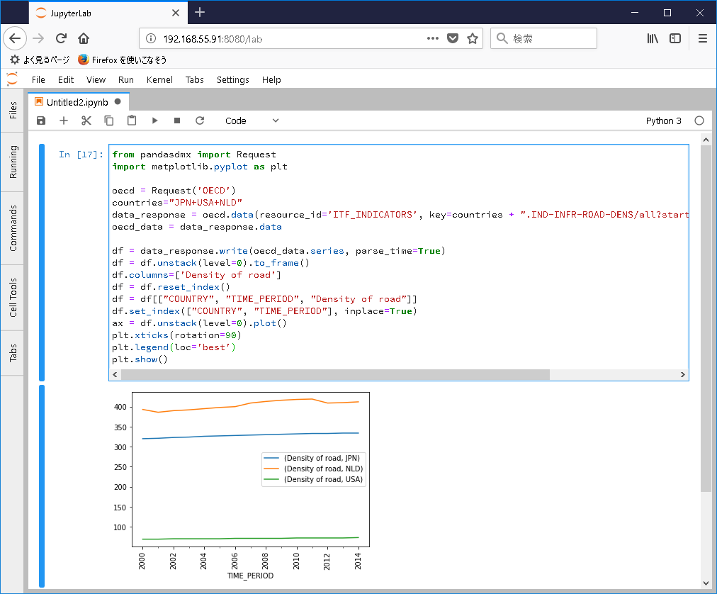
Jupyterとpandasdmxを使用して、OECDの道路密度データを取得する

Jupyterとpandasdmxを使用して、OECDの道路密度(Density of road, km per one hundred sq.km)データを取得してグラフ表示するには、以下のコードを実行します。

〇出力グラフ

〇コード

from pandasdmx import Request
import matplotlib.pyplot as plt

oecd = Request('OECD')
countries="JPN+USA+NLD"
data_response = oecd.data(resource_id='ITF_INDICATORS', key=countries + ".IND-INFR-ROAD-DENS/all?startTime=2000&endTime=2016")
oecd_data = data_response.data

df = data_response.write(oecd_data.series, parse_time=True)
df = df.unstack(level=0).to_frame()
df.columns=['Density of road']
df = df.reset_index()
df = df[["COUNTRY", "TIME_PERIOD", "Density of road"]]
df.set_index(["COUNTRY", "TIME_PERIOD"], inplace=True)
ax = df.unstack(level=0).plot()
plt.xticks(rotation=90)
plt.legend(loc='best')
plt.show()

〇元データ
Indicators
https://stats.oecd.org/Index.aspx?DataSetCode=ITF_INDICATORS


○関連情報
・Pandasdmxに関する他の記事はこちらを参照してください。

Jupyterとpandasdmxを使用して、OECDの道路人身事故データを取得する

Jupyterとpandasdmxを使用して、OECDの道路人身事故(Road injury accidents)データを取得してグラフ表示するには、以下のコードを実行します。

〇出力グラフ

〇コード

from pandasdmx import Request
import matplotlib.pyplot as plt

oecd = Request('OECD')
countries="JPN+USA+IND"
data_response = oecd.data(resource_id='ITF_ROAD_ACCIDENTS', key=countries + ".T-ACCI-TOT/all?startTime=1970&endTime=2016")
oecd_data = data_response.data

df = data_response.write(oecd_data.series, parse_time=True)
df = df.unstack(level=0).to_frame()
df.columns=['Injury accident']
df = df.reset_index()
df = df[["COUNTRY", "TIME_PERIOD", "Injury accident"]]
df.set_index(["COUNTRY", "TIME_PERIOD"], inplace=True)
ax = df.unstack(level=0).plot()
plt.xticks(rotation=90)
plt.legend(loc='best')
plt.show()

〇元データ
Road injury accidents
https://stats.oecd.org/Index.aspx?DataSetCode=ITF_ROAD_ACCIDENTS


○関連情報
・Pandasdmxに関する他の記事はこちらを参照してください。

Jupyterとpandasdmxを使用して、OECDの国内乗客輸送データを取得する

Jupyterとpandasdmxを使用して、OECDの国内乗客輸送(Inland passenger transport)データを取得してグラフ表示するには、以下のコードを実行します。

〇出力グラフ

〇コード

from pandasdmx import Request
import matplotlib.pyplot as plt

oecd = Request('OECD')
countries="JPN+USA+AUS"
data_response = oecd.data(resource_id='ITF_PASSENGER_TRANSPORT', key=countries + ".T-PASS-TOT-INLD/all?startTime=2000&endTime=2016")
oecd_data = data_response.data

df = data_response.write(oecd_data.series, parse_time=True)
df = df.unstack(level=0).to_frame()
df.columns=['Millions Passenger-kilometres']
df = df.reset_index()
df = df[["COUNTRY", "TIME_PERIOD", "Millions Passenger-kilometres"]]
df.set_index(["COUNTRY", "TIME_PERIOD"], inplace=True)
ax = df.unstack(level=0).plot()
plt.xticks(rotation=90)
plt.legend(loc='best')
plt.show()

〇元データ
Passenger transport
https://stats.oecd.org/Index.aspx?DataSetCode=ITF_PASSENGER_TRANSPORT


○関連情報
・Pandasdmxに関する他の記事はこちらを参照してください。

Jupyterとpandasdmxを使用して、OECDのコンテナ輸送データを取得する

Jupyterとpandasdmxを使用して、OECDのコンテナ輸送(Containers transport)データを取得してグラフ表示するには、以下のコードを実行します。

〇出力グラフ

〇コード

from pandasdmx import Request
import matplotlib.pyplot as plt

oecd = Request('OECD')
countries="GRC+BGR+DEU"
data_response = oecd.data(resource_id='ITF_GOODS_TRANSPORT', key=countries + ".T-CONT-RL-TEU/all?startTime=2000&endTime=2016")
oecd_data = data_response.data

df = data_response.write(oecd_data.series, parse_time=True)
df = df.unstack(level=0).to_frame()
df.columns=['TEU']
df = df.reset_index()
df = df[["COUNTRY", "TIME_PERIOD", "TEU"]]
df.set_index(["COUNTRY", "TIME_PERIOD"], inplace=True)
ax = df.unstack(level=0).plot()
plt.xticks(rotation=90)
plt.legend(loc='best')
plt.show()

〇元データ
Freight transport
https://stats.oecd.org/Index.aspx?DataSetCode=ITF_GOODS_TRANSPORT


○関連情報
・Pandasdmxに関する他の記事はこちらを参照してください。